skip to Main Content

I am trying to scrape information about orbits for asteroids in R. I have tried rvest and selectorgadget, however the website is dynamic. The website is: https://ssd.jpl.nasa.gov/tools/sbdb_lookup.html#/?sstr=2006%20WP1

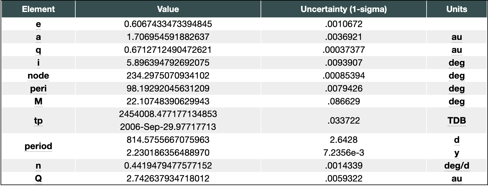
I am wanting to get the data for the Osculating Orbital Elements under the Orbit Parameters drop down shown here:
enter image description here

I am not very familiar with html or json, so I am looking for help downloading this table into R.

2

Answers


  1. Use their API.

    As an example of how to use the API, inspecting the page we can see the parameters used and recreate them (although I have changed it to use the direct identifier rather than a search string because it is quicker):

    # Query parameters
    params <- list(
      spk              = "3359266",
      `alt-des`        = 1,
      `alt-orbits`     = 1,
      `ca-data`        = 1,
      `ca-time`        = "both",
      `ca-tunc`        = "both",
      `cd-epoch`       = 1,
      `cd-tp`          = 1,
      discovery        = 1,
      `full-prec`      = 1,
      `nv-fmt`         = "both",
      `orbit-defs`     = 1,
      `phys-par`       = 1,
      `r-notes`        = 1,
      `r-observer`     = 1,
      `radar-obs`      = 1,
      sat              = 1,
      `vi-data`        = 1,
      www              = 1
    )
    
    # Make query string
    param_string <- paste0(names(params), "=", params, collapse = "&")
    

    Now retrieve the data:

    dat <- jsonlite::fromJSON(
      sprintf("https://ssd-api.jpl.nasa.gov/sbdb.api?%s", param_string)
      )
    
    # Inspect 
    dat$orbit$elements
    
           sigma  name                                                 title units                value  label
    1   .0010672     e                                          eccentricity  <NA>    .6067433473394845      e
    2   .0036921     a                                       semi-major axis    au    1.706954591882637      a
    3  .00037377     q                                   perihelion distance    au    .6712712490472621      q
    4   .0093907     i inclination; angle with respect to x-y ecliptic plane   deg    5.896394792692075      i
    5  .00085394    om                       longitude of the ascending node   deg    234.2975070934102   node
    6   .0079426     w                                argument of perihelion   deg    98.19292045631209   peri
    7    .086629    ma                                          mean anomaly   deg    22.10748390629943      M
    8    .033722    tp                            time of perihelion passage   TDB 2454008.477177134853     tp
    9       <NA> tp_cd                            time of perihelion passage   TDB 2006-Sep-29.97717713     tp
    10    2.6428   per                               sidereal orbital period     d    814.5755667075963 period
    11  .0014339     n                                           mean motion deg/d    .4419479477577152      n
    12  .0059322    ad                                     aphelion distance    au    2.742637934718012      Q
    
    Login or Signup to reply.
  2. To complete, using rvest read_html_live :

    ### Packages
    library(purrr)
    library(rvest)
    library(stringr)
    library(dplyr)
    
    Sys.setenv(
      CHROMOTE_CHROME = "C:\Program Files (x86)\Microsoft\Edge\Application\msedge.exe"
    )
    
    ### Parse and extract the table with html_live and XPath
    dd=read_html_live("https://ssd.jpl.nasa.gov/tools/sbdb_lookup.html#/?sstr=2006%20WP1")
    s=html_elements(dd,xpath = "(//table)[1]") %>% html_table()
    
    ### TP and period rows are merged. To fix this, we create new lines.
    rows=c("tp","period")
    labels=list(c("TDB","TDB"),c("d","y"))
    
    nasa=function(x,y){
      f=html_elements(dd,xpath = paste0('(//table)[1]//tr[contains(.,"',x,'")]/td[2]')) %>%
        html_text2() %>% 
      str_split(pattern = "n") %>%
        unlist()
      
      g=html_elements(dd,xpath = paste0('(//table)[1]//tr[contains(.,"',x,'")]/td[3]')) %>%
        html_text2() %>% 
        str_split(pattern = "n") %>%
        unlist()
      
    tibble(Element=x,Value=f,`Uncertainty (1-sigma)`=g, Units=y)
    }
    
    temp=map2(rows,labels,nasa)
    pp=bind_rows(temp)
    
    ### Merge the new lines with the table and delete old rows
    output=s[[1]] %>% 
      add_row(pp,.before = 8) %>%
      slice(-c(12,13))
    

    Output :

    # A tibble: 13 × 4
       Element Value                `Uncertainty (1-sigma)` Units  
       <chr>   <chr>                <chr>                   <chr>  
     1 e       0.6067433473394845   .0010672                ""     
     2 a       1.706954591882637    .0036921                "au"   
     3 q       0.6712712490472621   .00037377               "au"   
     4 i       5.896394792692075    .0093907                "deg"  
     5 node    234.2975070934102    .00085394               "deg"  
     6 peri    98.19292045631209    .0079426                "deg"  
     7 M       22.10748390629943    .086629                 "deg"  
     8 tp      2454008.477177134853 .033722                 "TDB"  
     9 tp      2006-Sep-29.97717713 .033722                 "TDB"  
    10 period  814.5755667075963    2.6428                  "d"    
    11 period  2.230186356488970    7.2356e-3               "y"    
    12 n       0.4419479477577152   .0014339                "deg/d"
    13 Q       2.742637934718012    .0059322                "au"  
    
    Login or Signup to reply.
Please signup or login to give your own answer.
Back To Top
Search