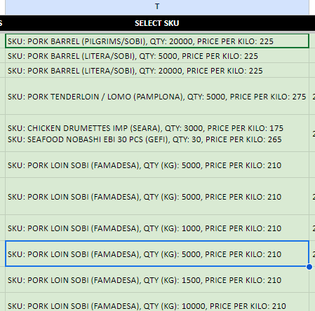
Currently I have this data format on my google sheet:
SKU: PORK BARREL (PILGRIMS/SOBI), QTY: 20000, PRICE PER KILO: 225
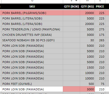
Then I want format my Data like this
Then I tried to format it using appscript this code
/**
 * Multiplies an input value by 2.
 * @param {number} input The number to double.
 * @return The input multiplied by 2.
 * @customfunction
*/
function DOUBLE(input) {
  return input * 2;
}
function result(range) {
  delimiter = ":"
  targetColumn = 19

  var output2 = [];
  for(var i=0, iLen=range.length; i<iLen; i++) {
    var s = range[i][targetColumn].split(delimiter);
    for(var j=0, jLen=s.length; j<jLen; j++) {
      var output1 = [];
      for(var k=0, kLen=range[0].length; k<kLen; k++) {
        if(k == targetColumn  ) {
          output1.push(s[j]);
        } else {
          output1.push(range[i][k]);
        }
      }
      output2.push(output1);
    }
  }
  return output2;
}
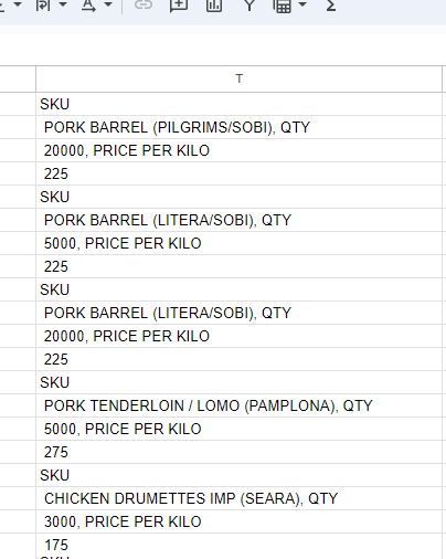
but my result is like this one
It goes vertical instead of horizontal.
How can we achieve it like on my desire output to be horizontal and segregate the data.
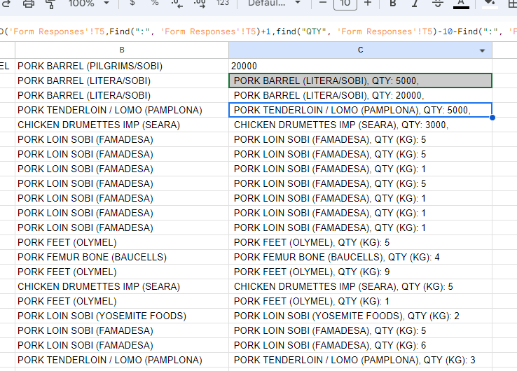
I also tried to do MID function to split the data but I’m having problem with the QTY , QTY(KG) , QTY(BOX)
I used this code
=MID('Form Responses'!T5,Find(":", 'Form Responses'!T5)+1,find("QTY", 'Form Responses'!T5)-10-Find(":", 'Form Responses'!T5)+20)


3
Answers
Can You Try this –
Since I only had one line of text data I just repeated it.
You can also try: